PI Deep Dive

Note

Looking for the function documentation? See PIMoveTo.

In this section the process for developing the PI controller is detailed. This includes deriving the kinematic relationships and creating trajectory profiles.

Derivation

Note

The derivation presented is a summary of the work by T.A. Baede, Motion control of an omnidirectional mobile robot (2006).

Essential to any advanced PID controller, the kinematic relationships and control laws were developed for a tri-omni wheel robot.

Kinematic Relationships

First, the robot’s location and heading with respect to the course’s (global) frame is defined as \((x, y, \theta)\). Additionally, the robot’s velocity with respect to the course’s frame is defined as \((\dot{x}, \dot{y}, \dot{\theta})\). With respect to the robot’s frame, the angles for wheels 1, 2, and 3 are \(a_1=30^\circ\), \(a_2=150^\circ\), and \(a_3=270^\circ\) respectively. Below is a picture of the robot’s local axis.

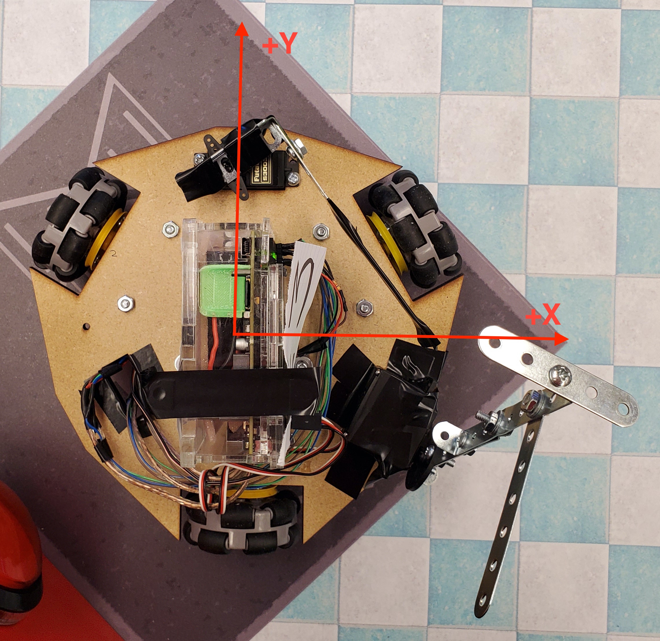
Next, the translational velocity of each wheel, \(v_i\) that make up the robot’s velocity can be split into its components:

\(v_i = v_{trans, i} + v_{rot}\tag{1}\label{eq:1}\)

Looking at \(v_{trans, i}\), we can map the vector onto \(\dot{x}\) and \(\dot{y}\) leading to the general equation for translation at each wheel:

\(v_{trans, i} = -\sin(\theta+a_i)\dot{x}+\cos(\theta+a_i)\dot{y}\tag{2}\)

Now consider the case were the robot only performs a rotation. Each wheel’s translational velocity, \(v_{rot}\), will have to be the following:

\(v_{rot}=R\dot{\theta}\tag{3}\)

where \(R\) is the radius from the center of the robot to the wheels. Note that each wheel will have the same equation as \(R\) is the same for all wheels. The value of \(R\) for our robot was measured to be 0.0869 meters.

Substituting the equations for \(v_{trans, i}\) and \(v_{rot}\) into the equation \(\eqref{eq:1}\), the following equation is created:

\(v_i=-\sin(\theta+a_i)\dot{x}+\cos(\theta+a_i)+R\dot{\theta}\tag{4}\label{eq:4}\)

This equation transforms the robot’s velocities into the translational velocity of each wheel. However, we can also relate the robot’s velocities into the angular velocity of each wheel as translational velocities are directly related to angular velocities:

\(v_i=r\dot{\phi_i}\tag{5}\label{eq:5}\)

where \(r\) is the radius of the wheels, measured to be 0.027 meters.

Substituting \(\eqref{eq:5}\) into \(\eqref{eq:4}\) and rearranging to solve for \(\dot{\phi}\), we get:

\(\dot{\phi}_i=\frac{1}{r}(-\sin(\theta+a_i)\dot{x}+\cos(\theta+a_i)+R\dot{\theta})\tag{6}\label{eq:6}\)

Converting \(\eqref{eq:6}\) from global coordinates to local coordinates is out-of-scope of the documentation (see Baede’s paper). However, the end result is the following equation for each wheel’s angular velocity given the robot’s velocities and steering in the local frame, defined as \([x_L, y_L]\):

\(\dot{\phi}_i=(-\sin(\theta+a_i)\cos(\theta)\dot{x}_L+\cos(\theta+a_i)\cos(\theta)\dot{y}_L+R\dot{\theta})/r\tag{7}\label{eq:7}\)

Control Laws

When controlling a robot, we will have an idea of the movement it should perform, called the reference movement. However, simply using \(\eqref{eq:7}\) to find the angular velocities of each wheel and setting each motor to the respective percent values will not suffice. This is because of effects such as friction and motor powers not being equivalent or consistent. Thus, it is neccessary to produce control laws to use for a feedback loop.

We can use \(\eqref{eq:7}\) to produce reference angular velocities of each wheel, \(\dot{\phi}_{ref,i}\), and through integration can also create reference angular positions of each wheel, \(\phi_{ref,i}\).

It was choosen to use a position controller as converting from encoder counts directly to angular postion is more likely to be more accurate rather than having to estimate an average velocity during program execution.

---

Control actions is calculated based on the difference between reference angular positions and actual angular positions:

\(e=\phi_{ref,i}-\phi_i\tag{8}\)

\(e\) is the tracking error. Note that the units for \(e\), \(\phi_{ref,i}\), and \(\phi_i\) are radians.

For use in a program, the discrete form of the PID control law is implemented:

\(u_k=K_pe_k+K_i\Delta T\sum_{j=1}^k e_j+\frac{K_d} {\Delta T}(e_k-e_{k-1})\tag{9}\)

\(u\)	Control signal
\(k\)	Control loop iteration
\(K_p\)	Proportional constant
\(K_i\)	Integral constant
\(K_d\)	Derivative constant
\(e\)	Tracking error
\(\Delta T\)	Time between interations

Note that for the final control loop, the derivative term was not implemented as it was found to be not neccessary.

Implementation

With the mathematical concepts defined, the code implementation can be constructed. Below is a flowchart of the implementation.

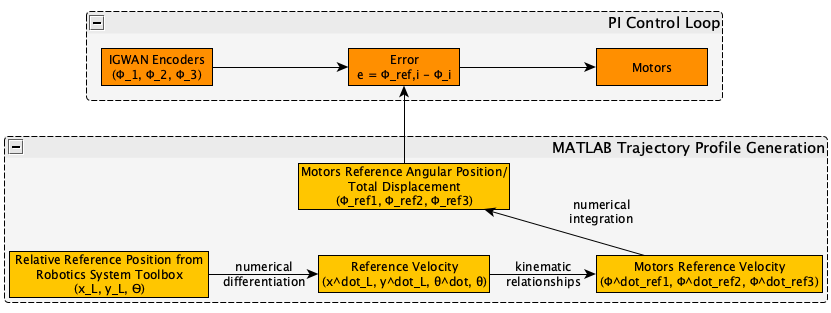
Trajectory profiles

To represent the reference angular positions, pre-generated trajectory profiles are generated for every movement. This is because the RPS has a large delay that negatively impacts the accuracy of the error, especially as the robot moves. To solve this, trajectory profiles are generated in MATLAB, using the code shown in Trajectory Profile Generation. Then the Proteus will read the profile file in the SD card, and store the reference values in an 2D array, which will be compared to in real time. Each trajectory profile outputted has the same format:

 0.000000        0.000000        0.000000        0.000000        0.000000        0.000000
 0.051794        0.051794        0.103589        -1.035885       -1.035885       2.071770
 0.192379        0.192379        0.384757        -1.775803       -1.775803       3.551606
 0.392157        0.392157        0.784313        -2.219754       -2.219754       4.439508
 0.621531        0.621531        1.243062        -2.367738       -2.367738       4.735475

From left to right, the columns are wheel 1’s, wheel 2’s, and wheel 3’s refererence total angular displacement, and wheel 1’s, wheel 2’s, and wheel 3’s refererence angular velocity. Although we only use total angular displacement to determine error, reference angular velocity is used to help decide which direction to wheels should spin in response to error as encoder counts can only increase.

To generate the reference values, the desired \(x_L\), \(y_L\), and \(\theta\) displacement values are first set along with their respective time stamps:

wpts = [0 0.5; 0 0.2; THETA THETA];

The above code sets the waypoints in a matrix, in the form [\(x_1~x_2 ... x_n\); \(~y_1~y_2 ... y_n\); \(~\theta_1~\theta_2 ... \theta_n\)] with the first waypoint always having 0 as the x and y values. It also sets the final waypoint 0.5 meters in the positive x and 0.2 meters in the positive y, with respect to the robot’s local frame. THETA can defined to be the offset of motor 1 from the local \(x_L\) axis. For our robot, THETA was defined as \(\pi/6\) such that motors 1 and 2 would move the robot forward. An offset can also be added to the \(\theta\) waypoint values so that the local frame of the robot can be rotated. For example, if the way points were:

wpts = [0 0.5; 0 0.2; THETA+pi/2 THETA+pi/2];

Then the robot’s local frame (with it’s x and y axis) is rotated 90 degrees counter-clockwise.

Next, the timestamps need to be set for each waypoint:

tpts = [0, 2];
tvec = 0:0.1:2;

tpts stores the timestamp in seconds for each waypoint. The first time is aways zero, and each waypoint must have it’s own timestamp. I.e, for \(n\) waypoints in wpts, there must be \(n\) timestamps in tpts. tvec stores the overall update rate of the trajectory profile and also the PID control loop. In the example above, there will be a reference value ever 0.1 seconds. Note that both tps and tvec must end with the same time value.

The displacement and timestamp values are passed into cubicpolytraj, part of the Robotics System Toolbox, which produces a cubic trajectory profile. We’re specifically interested in the reference positions and velocities, stored in q and qd respectively.

The kinematic relationship defined previously in equation \(\eqref{eq:7}\) is used to convert the generated reference velocities into reference angular velocities for each wheel:

phiVel1 = (-sin(q(3,:)+MOTOR_ANGLE_1).*cos(q(3,:)).*qd(1,:)+cos(q(3,:)+MOTOR_ANGLE_1).*cos(q(3,:)).*qd(2,:)+R.*qd(3,:))/r;
phiVel2 = (-sin(q(3,:)+MOTOR_ANGLE_2).*cos(q(3,:)).*qd(1,:)+cos(q(3,:)+MOTOR_ANGLE_2).*cos(q(3,:)).*qd(2,:)+R.*qd(3,:))/r;
phiVel3 = (-sin(q(3,:)+MOTOR_ANGLE_3).*cos(q(3,:)).*qd(1,:)+cos(q(3,:)+MOTOR_ANGLE_3).*cos(q(3,:)).*qd(2,:)+R.*qd(3,:))/r;

Now to convert the reference angular velocities into reference total angular displacment, numerical integration is performed using the following approximation based on the trapezoidal rule:

\(\phi_{ref}[i]=\phi_{ref}[i-1]+\frac{\Delta T}{2}(\dot{\phi}_{ref}[i]+\dot{\phi}_{ref}[i-1])\tag{10}\)

This formula is implemented in MATLAB as:

phiRef1(1) = 0;
phiRef2(1) = 0;
phiRef3(1) = 0;
for i=2:length(phiVel1)
    phiRef1(i)= phiRef1(i-1)+abs((DELTA_T/2)*(phiVel1(i)+phiVel1(i-1)));
    phiRef2(i)= phiRef2(i-1)+abs((DELTA_T/2)*(phiVel2(i)+phiVel2(i-1)));
    phiRef3(i)= phiRef3(i-1)+abs((DELTA_T/2)*(phiVel3(i)+phiVel3(i-1)));
end

Note that the initial total angular displacement is always set to 0. Also note the addition of an absolute value to the implementation. This is because encoder counts only can increase in our hardware, thus making the actual angular displacements always positive.

The reference total angular displacement values are then written to the output file

fileID = fopen(FILE_NAME,'w');
for i=1:length(phiRef1)
    fprintf(fileID, '%f\t%f\t%f\t%f\t%f\t%f\r\n', abs(phiRef1(i)), abs(phiRef2(i)), abs(phiRef3(i)), phiVel1(i), phiVel2(i), phiVel3(i));
    %fprintf(fileID, '%f\t%f\t%f\n', abs(phiRef1(i)), abs(phiRef2(i)), abs(phiRef3(i)));
end

which results in a output with format of the example trajectory profile shown above.

PI function

For your convenience, the code for the PID function is shown here:

Show/Hide PID Function Code

void PIMoveTo(char* fName, int size, bool preload) {

     /* Set important variables */
     int countNew1 = 0;
     int countNew2 = 0;
     int countNew3 = 0;
     int countOld1 = 0;
     int countOld2 = 0;
     int countOld3 = 0;
     float displacement1 = 0.0;
     float displacement2 = 0.0;
     float displacement3 = 0.0;
     float refSpeed1;
     float refSpeed2;
     float refSpeed3;
     float phiVel1 = 0.0;
     float phiVel2 = 0.0;
     float phiVel3 = 0.0;
     float phi1 = 0.0;
     float phi2 = 0.0;
     float phi3 = 0.0;
     float motorSpeed1 = 0.0;
     float motorSpeed2 = 0.0;
     float motorSpeed3 = 0.0;
     float errorTotal1 = 0.0;
     float errorTotal2 = 0.0;
     float errorTotal3 = 0.0;
     float Kp = 20.0;
     float Ki = 1.0;
     float Kd = 0.0;

     /* Get trajectory profile from file */
     FEHFile *fptr = SD.FOpen(fName,"r");
     /* Open write files to track error and delta angular displacement */
     // This is useful for tuning among other things
     FEHFile *fOutErrptr = SD.FOpen("errorLog.txt","w");
     FEHFile *fOutDispptr = SD.FOpen("dispLog.txt","w");
     FEHFile *fOutVelptr = SD.FOpen("velLog.txt","w");

     /* Init 2d arrays to store reference data and other temp variables to read from file */
     float pos_ref[3][size];
     float vel_ref[3][size];
     float temp1;
     float temp2;
     float temp3;
     /* If file failed to open, or invalid profile, return and make the screen red */
     if(SD.FEof(fptr)) {
         LCD.Clear(FEHLCD::Red);
         return;
     }
     /* Parse trajectory file */
     int i = 0;
     while(!SD.FEof(fptr)) {
         SD.FScanf(fptr, "%f%f%f%f%f%f", &temp1, &temp2, &temp3, &refSpeed1, &refSpeed2, &refSpeed3);
         pos_ref[0][i] = temp1;
         pos_ref[1][i] = temp2;
         pos_ref[2][i] = temp3;
         vel_ref[0][i] = refSpeed1;
         vel_ref[1][i] = refSpeed2;
         vel_ref[2][i] = refSpeed3;
         i++;
     }
     if(size < i) {
         LCD.Clear(FEHLCD::Red);
         return;
     }
     size = i;
     /* Close trajectory file */
     SD.FClose(fptr);
     /* PRELOAD LOOP */
     if(preload) {
         // Set green to show it's ready
         LCD.Clear(FEHLCD::Green);
         while(getCdsColor(true) == 0); // wait until a light turns on
     }
     /* Reset encoder counts */
     motor1_encoder.ResetCounts();
     motor2_encoder.ResetCounts();
     motor3_encoder.ResetCounts();
     /* PI LOOP */
     // Yes, not PID as the derivative term isn't needed currently
     for (int i = 0; i < size; i++) {
         /* Get new encoder counts */
         countNew1 = motor1_encoder.Counts();
         countNew2 = motor2_encoder.Counts();
         countNew3 = motor3_encoder.Counts();
         if(errorCurr1 < 0.0) {
             displacement1 = countsToRadDisp(countNew1, countOld1) * -1;
         } else {
             displacement1 = countsToRadDisp(countNew1, countOld1);
         }
         if(errorCurr2 < 0.0) {
             displacement2 = countsToRadDisp(countNew2, countOld2) * -1;
         } else {
             displacement2 = countsToRadDisp(countNew2, countOld2);
         }
         if(errorCurr3 < 0.0) {
             displacement3 = countsToRadDisp(countNew3, countOld3) * -1;
         } else {
             displacement3 = countsToRadDisp(countNew3, countOld3);
         }
         // Set old counts to new counts for the next iteration
         countOld1 = countNew1;
         countOld2 = countNew2;
         countOld3 = countNew3;
         // Add to total angular displacement
         phi1 += displacement1;
         phi2 += displacement2;
         phi3 += displacement3;

         // Write to log file
         SD.FPrintf(fOutDispptr, "%f\t%f\t%f\n", displacement1, displacement2, displacement3);

         /* Calculate current error relative to reference angular positions for each encoder */
         errorCurr1 = pos_ref[0][i] - phi1;
         errorCurr2 = pos_ref[1][i] - phi2;
         errorCurr3 = pos_ref[2][i] - phi3;

         // Saftey check in case something goes terribly wrong, may or may not be needed later
         if(errorCurr1 > 3)
             return;


         // Write errors to log file
         SD.FPrintf(fOutErrptr, "%f\t%f\t%f\n", errorCurr1, errorCurr2, errorCurr3);
         // Add to total error (for integral term)
         errorTotal1 += errorCurr1;
         errorTotal2 += errorCurr2;
         errorTotal3 += errorCurr3;

         /* Calc motor speeds (rad/s) using P and I */
         motorSpeed1 = Kp * errorCurr1 + Ki * DELTA_T * (errorTotal1);
         motorSpeed2 = Kp * errorCurr2 + Ki * DELTA_T * (errorTotal2);
         motorSpeed3 = Kp * errorCurr3 + Ki * DELTA_T * (errorTotal3);

         /* Use the reference velocities to determine if motor speed should change signs */
         if(vel_ref[0][i] < 0.0 || (errorCurr1 < 0 && motorSpeed1 < 0)) {
             motorSpeed1 *= -1.0;
         }
         if(vel_ref[1][i] < 0.0 || (errorCurr2 < 0 && motorSpeed2 < 0)) {
             motorSpeed2 *= -1.0;
         }
         if(vel_ref[2][i] < 0.0 || (errorCurr3 < 0 && motorSpeed3 < 0)) {
             motorSpeed3 *= -1.0;
         }

         SD.FPrintf(fOutVelptr, "%f\t%f\t%f\n", motorSpeed1, motorSpeed2, motorSpeed3);
         /* Set motors to speed */
         setRadSToPercent(motorSpeed1, motorSpeed2, motorSpeed3);
         /* Wait 0.1 seconds (100 miliseconds) */
         Sleep(100);
     }
     /* Done with trajectory profile, stop all motors */
     allStop();
     /* Close all log files */
     SD.FClose(fOutErrptr);
     SD.FClose(fOutDispptr);
     SD.FClose(fOutVelptr);
 }

First, the values are read from the given trajectory file and stored in the respective 2D arrays:

 /* Parse trajectory file */
 int i = 0;
 while(!SD.FEof(fptr)) {
     SD.FScanf(fptr, "%f%f%f%f%f%f", &refPos1, &refPos2, &refPos3, &refSpeed1, &refSpeed2, &refSpeed3);
     pos_ref[0][i] = refPos1;
     pos_ref[1][i] = refPos2;
     pos_ref[2][i] = refPos3;
     vel_ref[0][i] = refSpeed1;
     vel_ref[1][i] = refSpeed2;
     vel_ref[2][i] = refSpeed3;
     i++;
 }

The 2D arrays are allocated such that the columns represents each motor and the rows each 0.1s value. pos_ref stores the reference positions, and the vel_ref stores the reference velocities to help determine which direction the motors should spin.

Next, if the preload argument is set to true, it will then wait until getCdsColor detects a light. Then, the motors encoders are reset:

 /* PRELOAD LOOP */
 if(preload) {
     // Set green to show it's ready
     LCD.Clear(FEHLCD::Green);
     while(getCdsColor(true) == 0); // wait until a light turns on
 }
 /* Reset encoder counts */
 motor1_encoder.ResetCounts();
 motor2_encoder.ResetCounts();
 motor3_encoder.ResetCounts();

And now the PI control loop starts. The first action is to get the number of encoder counts from each motor. Note the first iteration will always make these 0. However, for all other iterations, they will always be larger than the previous counts, stored in countOld(i).

 /* Get new encoder counts */
 countNew1 = motor1_encoder.Counts();
 countNew2 = motor2_encoder.Counts();
 countNew3 = motor3_encoder.Counts();

Next, countsToRadDisp will be called to convert the difference between the current and previous iteration encoder counts to angular displacement in radians. Note that depending on each motors previous error (0 for the first iteration), it may be inversed. This is another way to help account for the fact that the encoder counts can only increase.

 if(errorCurr1 < 0.0) {
     displacement1 = countsToRadDisp(countNew1, countOld1) * -1;
 } else {
     displacement1 = countsToRadDisp(countNew1, countOld1);
 }
 if(errorCurr2 < 0.0) {
     displacement2 = countsToRadDisp(countNew2, countOld2) * -1;
 } else {
     displacement2 = countsToRadDisp(countNew2, countOld2);
 }
 if(errorCurr3 < 0.0) {
     displacement3 = countsToRadDisp(countNew3, countOld3) * -1;
 } else {
     displacement3 = countsToRadDisp(countNew3, countOld3);
 }

Now we are done using the previous iteration values, so we can set the old counts to the new counts, and then add to our current total angular displacement.

 // Set old counts to new counts for the next iteration
 countOld1 = countNew1;
 countOld2 = countNew2;
 countOld3 = countNew3;
 // Add to total angular displacement
 phi1 += displacement1;
 phi2 += displacement2;
 phi3 += displacement3;

It is now time to calculate the current error (in radians), and increment the total error. Note that during this process, various values are written onto files in the SD Card. This is to help debug and tune the controller.

 /* Calculate current error relative to reference angular positions for each encoder */
 errorCurr1 = pos_ref[0][i] - phi1;
 errorCurr2 = pos_ref[1][i] - phi2;
 errorCurr3 = pos_ref[2][i] - phi3;

 /* ... */

 // Add to total error (for integral term)
 errorTotal1 += errorCurr1;
 errorTotal2 += errorCurr2;
 errorTotal3 += errorCurr3;

Then comes the PI equation, where we calculate the motor speeds to correct for the error, in rad/s. These values are also checked with the reference velocity and current error to help determing which way the motors should spin.

 /* Calc motor speeds (rad/s) using P and I */
 motorSpeed1 = Kp * errorCurr1 + Ki * DELTA_T * (errorTotal1);
 motorSpeed2 = Kp * errorCurr2 + Ki * DELTA_T * (errorTotal2);
 motorSpeed3 = Kp * errorCurr3 + Ki * DELTA_T * (errorTotal3);

 /* Use the reference velocities to determine if motor speed should change signs */
 if(vel_ref[0][i] < 0.0 || (errorCurr1 < 0 && motorSpeed1 < 0)) {
     motorSpeed1 *= -1.0;
 }
 if(vel_ref[1][i] < 0.0 || (errorCurr2 < 0 && motorSpeed2 < 0)) {
     motorSpeed2 *= -1.0;
 }
 if(vel_ref[2][i] < 0.0 || (errorCurr3 < 0 && motorSpeed3 < 0)) {
     motorSpeed3 *= -1.0;
 }

Finally, setRadSToPercent is called to set the motors to the correct percents from the given speeds in radians per second. Also not that this function does use the errCurr(i) variables (hence why they are global) to further help determine which direction the motors should spin. Then the loop waits 0.1 seconds before starting the next iteration.

 /* Set motors to speed */
 setRadSToPercent(motorSpeed1, motorSpeed2, motorSpeed3);
 /* Wait 0.1 seconds (100 miliseconds) */
 Sleep(100);

MATLAB Error Plotting and Caveats

Note

The MATLAB code to generate the plots is shown in Error Plotting and Trajectory Profile Generation.

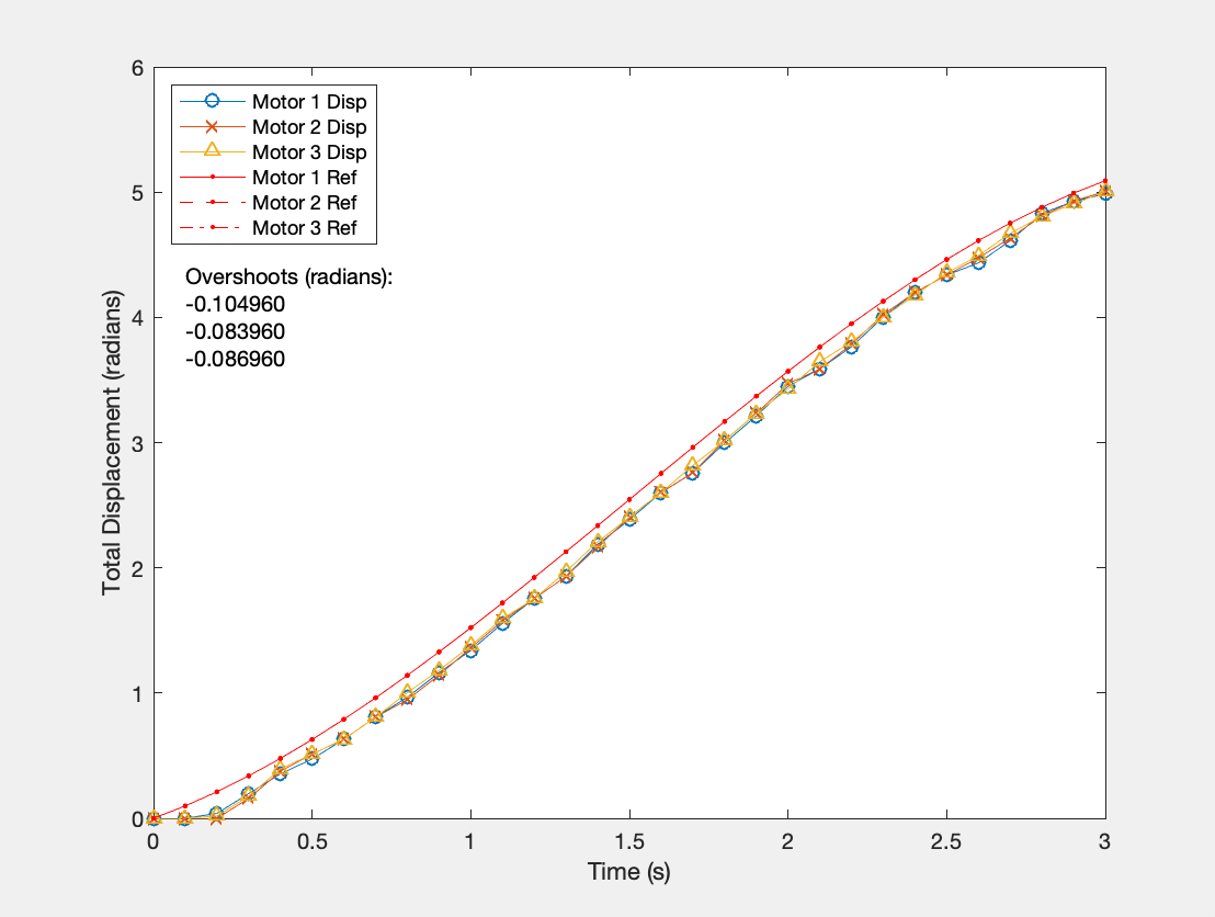
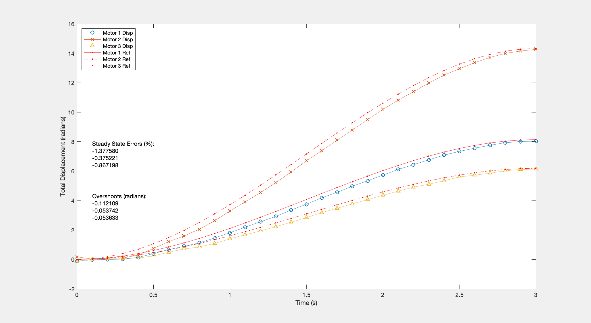
To generate the error plots, all one needs to do is input the error log files with the respective generated trajectory file name. Examples are given below.

Total displacement plot for a rotation

Total displacement plot for a translation in the x and y axis

Error plot for a translation in the x and y axis

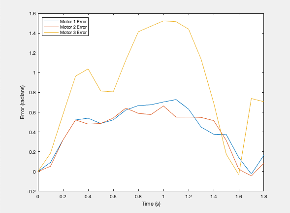
For all movements, the steady state error (end error) is very low which shows that our proportional constant of 20 and integral constant of 1 is very suitable. And no derivative term was added because of the accuracy.

However, as you may have noticed from reading the previous sections, determining which direction the motors should spin is a large issue as encoder counds can only increase. This is why undershoots are preferred over overshoots - the PI controller cannot accurately account for overshoots as well as undershoots. This is also why when generating the trajectory profiles, steps must be taken to make sure that the total displacement always increases. Take the following plots that show a bit of the trajectory profile generation process for example.

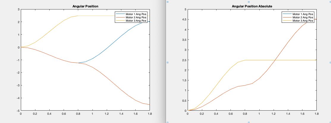
On the left is a plot of the “raw” total angular displacement reference values for each motor. It can be seen that motors 1 and 2 both decrease at multiple points in time. This is of course, impossible. So to account for the fact that encoder counts can only increase, we must take the absolute value of each angular displacement, shown on the right. However, you may notice that while on the original plot, motor 1 and 2 have different curves, on the absolute value plot, they have the same curve. This creates a clear problem as now both motors will act identical when in reality they shouldn’t. One step to fix this issue is to introduce angular velocity reference values, which can be both positive and negative. The plot is shown below.

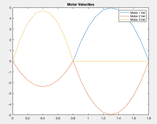
We can now see that there is a clear difference between all three motor curves which is good. Thus using the sign of the reference velocity can help determine which direction the motor should spin. However, we then must take into account for how the PI controller should respond to error. If it overshoots, then the motor must spin the opposite direction and vice versa. However, what if the reference velocity is negative? Then we negate the given displacement, but the motor ends up spinning in the wrong direction, only increasing error until the motor spins at 100% power. Thus more complicated checks had to be implemented in both the PIMoveTo and setRadSToPercent functions. But, these are still not perfect, and the PI controller does not respond as well to overshoots compared to undershoots. For this reason, when using this implementation, try to stick to a bit of overshoots.

And one final caveat to consider - it cannot account for wheels slipping. There are some interesting papers that look into using the coefficient of friction and the current angular velocity to compare with theorectical angular velocity, which then can determine if the wheels slip, but we did not have time to investigate it further.

If you made it this far, congrats! Hopefully you learned a lot more about of PI (and PID) controllers work.